Assessing Pre-training Bias with AWS SageMaker Clarify

Introduction

In the previous article, we discussed why explaining machine learning (ML) models is as important as their performance and how it benefits all the stakeholders. Now, we are going to see what explainability and fairness of ML models require in practice. Before trying to explain an ML model, we need to make sure that the data we feed to the model reflects the information that we wish the model to learn properly. To this end, we need to analyze the input dataset to determine if any biased information exists in the data and act accordingly to reduce those biases.

In this post, we are going to analyze a dataset using AWS SageMaker Clarify. We will discuss the implementation of SageMaker Clarify bias measures and their interpretations. The experiments are done in the AWS SageMaker environment, but you can implement these measures regardless of your coding environment.

You can find the Jupyter notebook of the experiments in this GitHub repository.

What is pre-training bias?

Since machine learning models look for certain patterns in the dataset, their performance depends on the quality of the data that was fed to them. If a dataset contains features/labels with imbalanced distributions, it will serve as a signal for the model to adapt its parameters in a way to reflect this imbalanced information.

However, In real-world applications the data doesn’t necessarily represent the patterns that we want models to learn. The datasets may be biased toward certain features or groups of features that only correlate with our desired output and have no causal relationship with the phenomena that we wish to model. These biases can force the model to deviate towards those unbalanced features and consequently favor certain features against others. This situation will become critical especially when the unbalanced features represent information that will impact certain groups of people, making the ML model’s prediction unfair.

A machine learning system is considered to be biased if it favors/disfavors certain groups of individuals. So, it is very important to check for biases in the dataset and employ bias reduction techniques prior to feeding the data to the model.

For example, consider an ML-based application that will assess people’s financial information and decide whether they are suitable for loans or not. In this case, the dataset on which the model is trained, may favor certain groups of people and this will cause the model to reduce the chances for others getting the loan.

By determining the existence of pre-training bias in the dataset, we want to detect the lack of balance in the dataset and mitigate them as much as we can, so the ML models can be trained on a fair dataset.

Getting the dataset

For the experiments, we are going to download the “Bank Marketing Data Set” from the UCI Machine Learning Repository. The dataset contains data regarding direct marketing campaigns of a Portuguese banking institution. The dataset consists of 41188 samples each of which has 21 attributes. These attributes are related to the clients, information about the last contacts of the current campaign, social and economic context information, and the output variable which indicates the conversion of the client. For the sake of simplicity, we will only consider the bank clients’ data along with the target variable. For a more thorough understanding of the dataset, please refer to this paper by Moro et al. 2014.

Let’s examine this dataset to see if any potential biases exist in it.

Experimental setup

Before jumping into the experiments, go ahead and download the dataset from here. We will use the data contained in bank-additional-full.csv and store it in an S3 bucket for later use. Since we are going to use SageMaker Clarify to detect potential biases in our dataset, it is convenient to conduct the experiments in a Jupyter notebook in the SageMaker environment. So, let’s open a SageMaker Jupyter notebook and start coding. First, let’s get the SageMaker session and its corresponding region. Also, we need a role for further use of AWS resources. We will also use the Boto3 S3 client to download the dataset from S3.

from sagemaker import Session
from sagemaker import get_execution_role
import boto3

session = Session()
region = session.boto_region_name
role = get_execution_role()
s3_client = boto3.client("s3")

Go ahead and download the dataset from S3 into the SageMaker environment. We are now ready to explore the dataset and compute the bias measures for its features.

Detecting pre-training bias in the dataset using SageMaker Clarify

Here, we are going to see if any possible biases exist in the dataset. SageMaker Clarify makes it easy to run bias detection jobs on datasets and computes various bias measures automatically.

Let’s first read the downloaded data using a Pandas dataframe.

import pandas as pd


# initial columns
bank_client_attributes_names = ['age', 'job', 'marital', 'education', 'default', 'housing', 'loan']
target_attribute_name = ['y']
col_names = bank_client_attributes_names + target_attribute_name
data_path = 'bank-additional-full.csv'
df = pd.read_csv(data_path, delimiter=';', index_col=None)
df = df[col_names]

As we said earlier, we only use attributes of bank client data. These attributes are age, job, marital, education, default, housing, and loan. We will use these attributes to develop a model for predicting the target variable which indicates whether the client subscribes to the bank offer or not. For a description of each of these attributes refer to the dataset repository.

Here is what the head of the Dataframe looks like:

  age        job  marital    education  default housing loan   y
0   56  housemaid  married     basic.4y       no      no   no  no
1   57   services  married  high.school  unknown      no   no  no
2   37   services  married  high.school       no     yes   no  no
3   40     admin.  married     basic.6y       no      no   no  no
4   56   services  married  high.school       no      no  yes  no

Let’s save and upload the client information subset of the dataframe into S3.

from sagemaker.s3 import S3Uploader
from sagemaker.inputs import TrainingInput

bucket = '<YOUR_S3_BUCKET>'
prefix = '<SOME_PREFIX>'

df.to_csv('df.csv', index=False)
df_uri = S3Uploader.upload("df.csv", "s3://{}/{}".format(bucket, prefix))

Now, let’s use SageMaker Clarify to run a pre-training bias detection job on the Dataframe we just uploaded to S3. To this end, first we need to import the clarify package from sagemaker. After that, we will define a processor for the job using clarify.SageMakerClarifyProcessor, which takes as input the SageMaker execution role and session, type and number of instances for the job, and a job prefix. We then specify the S3 path in which we want to save the pre-training bias detection results using bias_report_output_path. In order to run the job, we have to define two clarify objects, namely a DataConfig object, and a BiasConfig object.

The DataConfig object specifies the input and result data paths, features and target variable names, and the dataset type.

The BiasConfig object configures the options of the pre-training bias detection job. Here, we set label_values_or_threshold=['yes'] to indicate the positive outcome of bank customers who accepted the bank’s offer. We also set the facet_name to the list of all feature names to indicate that we want to examine all the features for the bias detection job.

Finally, we call the clarify_processor.run_pre_training_bias() function with the DataConfig and BiasConfig objects as its arguments to run the job. This will take several minutes depending on the size of the data and the type and number of processing instances of the clarify_processor. After the job is finished, the report is saved in the S3 in the bias_report_output_path.

from sagemaker import clarify

clarify_processor = clarify.SageMakerClarifyProcessor(
    role=role,
    instance_count=1,
    instance_type="ml.m5.xlarge",
    sagemaker_session=session,
    job_name_prefix='clarify-pre-training-bias-detection-job'
)

bias_report_output_path = "s3://{}/{}/clarify-bias".format(bucket, prefix)

bias_data_config = clarify.DataConfig(
    s3_data_input_path=df_uri,
    s3_output_path=bias_report_output_path,
    label="y",
    headers=df.columns.to_list(),
    dataset_type="text/csv",
)

bias_config = clarify.BiasConfig(
    label_values_or_threshold=['yes'],
    facet_name=['age', 'job', 'marital', 'education', 'default', 'housing', 'loan'],
)

clarify_processor.run_pre_training_bias(
    data_config=bias_data_config,
    data_bias_config=bias_config
)

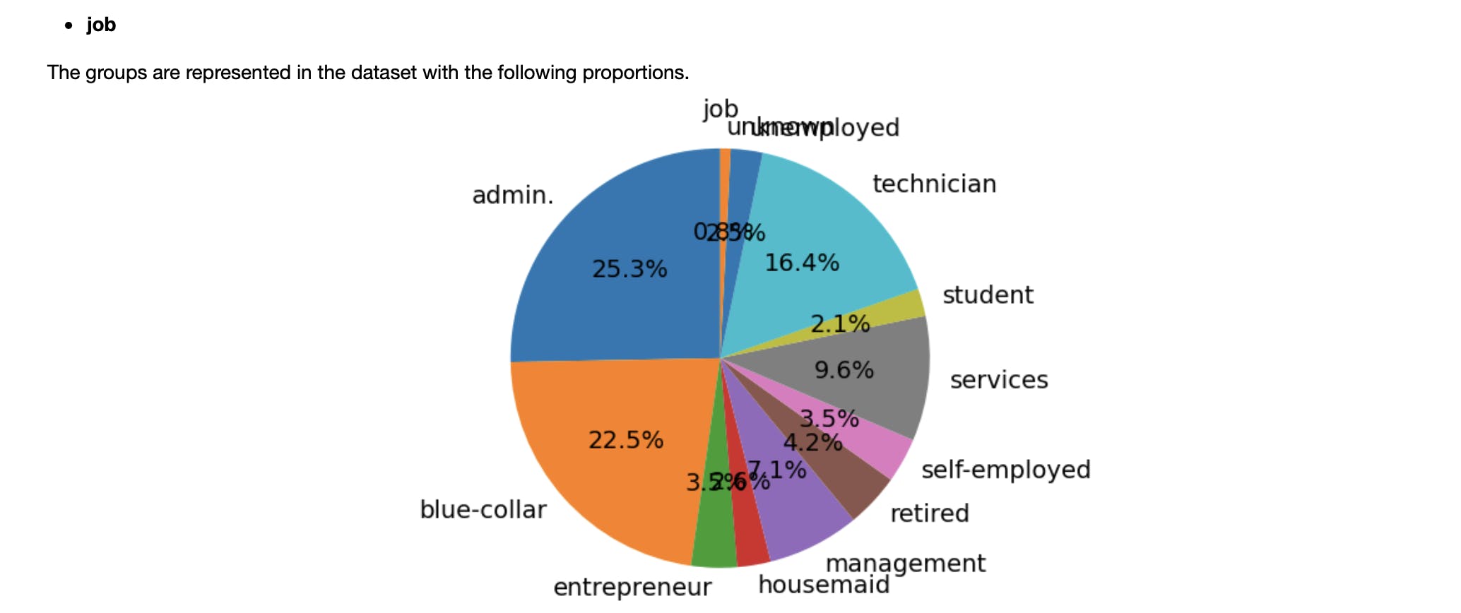
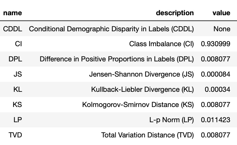
Clarify computes several metrics for detecting the pre-training bias in the dataset. These metrics depend on the distribution of each feature and the posterior probability of the target variable given each value of the feature. For more information regarding the terminology and definition of terms used by Clarify, please read the official documentation.

Here is the screenshot of how the report file looks like for the “job” feature:

A pie chart indicating the histogram of feature

A table of the clarify report for

Now, let’s elaborate more on each bias metric.

Class Imbalance (CI)

According to SageMaker Clarify documentation, the class imbalance metric is defined as $$ CI = \frac{n_a - n_d}{n_a + n_d}, $$

where $n\_a$ and $n\_d$ denote the number of observed labels for the favored and disfavored feature values, respectively. Let’s compute this metric by ourselves to have a more clear understanding of what these numbers represent.

Suppose we want to compute the class imbalance metric for people whose jobs are self-employed. First, we can see that around 3.5 % of the people on our dataset are self-employed.

ratio = len(df[df['job'] == 'self-employed']) / len(df)
print(100 * ratio)

3.450033990482665

This suggests that self-employed people may have been underrepresented in our dataset.

For computing the class imbalance for self-employed people, we are going to regard the number of people who are self-employed as $n\_d$, and the number of people who are not self-employed as $n\_a$. This is because we want to check that if the self-employed people are the disadvantaged group. Obviously, the sum of these two numbers equal the number of dataset samples. Defining $n\_d$ and $n\_a$, we are ready to compute the class imbalance:

def class_imbalance(df: pd.DataFrame, feature_name: str, feature_value: str) -> float:
    n_d = len(df[df[feature_name] == feature_value])
    n_a = len(df[df[feature_name] != feature_value])
    ci = (n_a - n_d)/(n_a + n_d)
    return ci

print(class_imbalance(df, 'job', 'self-employed'))

0.9309993201903467

Which is the same as the CI metric for job feature with value self-employed in the report file which was computed by SageMaker Clarify.

This number means that the difference between the number of self-employed and not self-employed people is 93% of the entire population. In an ideal situation where CI is equal to zero, there would be an equal number of self-employed and non-self-employed people in the dataset.

The $CI=0.93$ suggests that a model trained on this data, may favor non-self-employed people more (indicated by $n\_a$ in the formula), and we should use the model’s output for self-employed people in a more cautious way.

Difference in Positive Proportions in Labels (DPL)

According to the SageMaker Clarify documentation, the DPL metric is defined as the $$ DPL = q_a - q_d, $$

Where $q\_a=n\_a^{(1)}/n\_a=$P(positive label | favored feature value) and $q\_d=n\_d^{(1)}/n\_d=$P(positive label | disfavored feature value), and the superscript (1) denotes the subset of samples that have a positive label for their class. Let’s implement it and see that our results agree with the report file:

def dpl(df: pd.DataFrame, feature_name: str, feature_value: str, label_name: str, label_value:str) -> float:
    n_d = len(df[df[feature_name] == feature_value])
    n_a = len(df[df[feature_name] != feature_value])

    # p(label_value|not feature_value) or q_a
    p_positive_given_a = len(
        df[(df[feature_name] != feature_value) & (df[label_name] == label_value)]
    ) / n_a

    # p(label_value|feature_value) or q_d
    p_positive_given_d = len(
        df[(df[feature_name] == feature_value) & (df[label_name] == label_value)]
    ) / n_d
    return p_positive_given_a - p_positive_given_d

print(dpl(df, 'job', 'self-employed', 'y', 'yes'))

0.008077098359025064

As it is obvious from the code and the formula, this metric shows the difference between the probability of non-self-employed people with positive class and the probability of self-employed people with positive class.

Numbers close to zero indicate that two disjoint groups of people have the same proportion of positive class samples, whereas positive or negative numbers with large absolute value, indicates that people in group a or people in group d have a higher proportion of positive outcomes. We should be careful in using datasets with high DPL values for different groups since it may cause bias in the model training.

Kullback-Leibler Divergence (KL)

The KL divergence is a statistic for probability distributions and measures the relative entropy between two probability distributions. You can check the wikipedia article for a thorough explanation. Note that this measure is not symmetric. Let’s compute the KL divergence for self-employed people according to SageMaker Clarify documentation:

import numpy as np

def kl_divergence(
    df: pd.DataFrame,
    feature_name: str,
    feature_value: str,
    label_name: str,
    positive_label_value: str,
    negative_label_value: str
) -> float:
    n_d = len(df[df[feature_name] == feature_value])
    n_a = len(df[df[feature_name] != feature_value])

    p_positive_given_d = len(
        df[(df[feature_name] == feature_value) & (df[label_name] == positive_label_value)]
    ) / n_d
    p_negative_given_d = len(
        df[(df[feature_name] == feature_value) & (df[label_name] == negative_label_value)]
    ) / n_d

    p_positive_given_a = len(
        df[(df[feature_name] != feature_value) & (df[label_name] == positive_label_value)]
    ) / n_a
    p_negative_given_a = len(
        df[(df[feature_name] != feature_value) & (df[label_name] == negative_label_value)]
    ) / n_a

    kl_pa_pd = p_positive_given_a * np.log(p_positive_given_a/p_positive_given_d) + p_negative_given_a * np.log(p_negative_given_a/p_negative_given_d)
    return kl_pa_pd
print(kl_divergence(df, 'job', 'self-employed', 'y', 'yes', 'no'))

0.00033994894805770663

The KL statistic shows how much the dataset’s posterior distributions of being in the positive class for the self-employed and non-self-employed people are close to each other. The KL range of values are in the interval $\[0, \\infty)$. Values near zero mean the outcomes are similarly distributed for the different facets, and, positive values mean the label distributions diverge, the more positive the larger the divergence.

Jensen-Shannon Divergence (JS)

The JS divergence is based on KL divergence, but, it is a symmetric measure, i.e., given two probability distributions, $JS(p, q)=JS(q, p)$. The formula for computing JS divergence is as follows: $$ JS = \frac{1}{2}(KL(P_a || P) + KL(P_d || P)), $$

where $P=\\frac{1}{2}(P\_a + P\_d)$. Let’s implement this measure according to SageMaker Clarify documentation.

def js_divergence(
    df: pd.DataFrame,
    feature_name: str,
    feature_value: str,
    label_name: str,
    positive_label_value: str,
    negative_label_value: str
) -> float:
    n_d = len(df[df[feature_name] == feature_value])
    n_a = len(df[df[feature_name] != feature_value])

    p_positive_given_d = len(
        df[(df[feature_name] == feature_value) & (df[label_name] == positive_label_value)]
    ) / n_d
    p_negative_given_d = len(
        df[(df[feature_name] == feature_value) & (df[label_name] == negative_label_value)]
    ) / n_d

    p_positive_given_a = len(
        df[(df[feature_name] != feature_value) & (df[label_name] == positive_label_value)]
    ) / n_a
    p_negative_given_a = len(
        df[(df[feature_name] != feature_value) & (df[label_name] == negative_label_value)]
    ) / n_a

    p_positive = 0.5 * (p_positive_given_a + p_positive_given_d)
    p_negative = 0.5 * (p_negative_given_a + p_negative_given_d)

    term1 = p_positive_given_a * np.log(p_positive_given_a/p_positive) + p_negative_given_a * np.log(p_negative_given_a/p_negative)
    term2 = p_positive_given_d * np.log(p_positive_given_d/p_positive) + p_negative_given_d * np.log(p_negative_given_d/p_negative)
    return 0.5 * (term1 + term2)

print(js_divergence(df, 'job', 'self-employed', 'y', 'yes', 'no'))

8.405728506055265e-05

The range of JS values is the interval $\[0, \\ln(2))$, where values near zero mean the labels are similarly distributed whereas positive values mean the label distributions diverge, the more positive the larger the divergence. This metric indicates whether there is a big divergence in one of the labels across facets.

Kolmogorov-Smirnov Distance (KS)

According to SageMaker Clarify documentation, The KS statistic is computed as the maximum divergence of label between distributions between features of an interested group and its complement in the dataset. The formula for computing the KS distance is as follows: $$ KS = \max(|P_a(y) - P_d(y)|), $$

where $P\_a(y)$\=P(label y|feature value a). Let’s implement this statistic:

def ks_distance(
    df: pd.DataFrame,
    feature_name: str,
    feature_value: str,
    label_name: str,
    positive_label_value: str,
    negative_label_value: str
) -> float:
    n_d = len(df[df[feature_name] == feature_value])
    n_a = len(df[df[feature_name] != feature_value])

    p_positive_given_d = len(
        df[(df[feature_name] == feature_value) & (df[label_name] == positive_label_value)]
    ) / n_d
    p_negative_given_d = len(
        df[(df[feature_name] == feature_value) & (df[label_name] == negative_label_value)]
    ) / n_d

    p_positive_given_a = len(
        df[(df[feature_name] != feature_value) & (df[label_name] == positive_label_value)]
    ) / n_a
    p_negative_given_a = len(
        df[(df[feature_name] != feature_value) & (df[label_name] == negative_label_value)]
    ) / n_a

    ks_distance = np.max([np.abs(p_positive_given_a - p_positive_given_d), np.abs(p_negative_given_a - p_negative_given_d)])
    return ks_distance

print(ks_distance(df, 'job', 'self-employed', 'y', 'yes', 'no'))

0.008077098359025148

The range of KS distance values is in the interval $\[0, +1\]$, where values near zero indicate the labels were evenly distributed between feature values in all outcome categories, and, values near one indicate the labels for one outcome were all in one feature value, and finally, intermittent values indicate relative degrees of maximum label imbalance.

L-p norm (LP)

The L-p norm metric measures the sum of L-norm of the posterior distributions of positive and negative classes of the interested group given the feature value and its complement. Let’s implement this measure according to SageMaker Clarify documentation. As you can see, the default norm for this measure is the Euclidean or L-2 norm.

def lp_norm(
    df: pd.DataFrame,
    feature_name: str,
    feature_value: str,
    label_name: str,
    positive_label_value: str,
    negative_label_value: str
) -> float:
    n_d = len(df[df[feature_name] == feature_value])
    n_a = len(df[df[feature_name] != feature_value])

    p_positive_given_d = len(
        df[(df[feature_name] == feature_value) & (df[label_name] == positive_label_value)]
    ) / n_d
    p_negative_given_d = len(
        df[(df[feature_name] == feature_value) & (df[label_name] == negative_label_value)]
    ) / n_d

    p_positive_given_a = len(
        df[(df[feature_name] != feature_value) & (df[label_name] == positive_label_value)]
    ) / n_a
    p_negative_given_a = len(
        df[(df[feature_name] != feature_value) & (df[label_name] == negative_label_value)]
    ) / n_a

    lp = np.power((p_positive_given_d - p_positive_given_a)**2 + (p_negative_given_d - p_negative_given_a)**2, 0.5)
    return lp

print(lp_norm(df, 'job', 'self-employed', 'y', 'yes', 'no'))

0.011422742043954775

The range of LP values is the interval $\[0, \\sqrt{2})$, where values near zero mean the labels are similarly distributed, whereas positive values mean the label distributions diverge, the more positive the larger the divergence.

Total Variation Distance (TVD)

According to SageMaker Clarify documentation, the TVD is actually the sum of L-1 norms of the posterior distributions of positive and negative classes of the interested group given the feature value and its complement. Here is the implementation of TVD:

def tvd(
    df: pd.DataFrame,
    feature_name: str,
    feature_value: str,
    label_name: str,
    positive_label_value: str,
    negative_label_value: str
) -> float:
    n_d = len(df[df[feature_name] == feature_value])
    n_a = len(df[df[feature_name] != feature_value])

    p_positive_given_d = len(
        df[(df[feature_name] == feature_value) & (df[label_name] == positive_label_value)]
    ) / n_d
    p_negative_given_d = len(
        df[(df[feature_name] == feature_value) & (df[label_name] == negative_label_value)]
    ) / n_d

    p_positive_given_a = len(
        df[(df[feature_name] != feature_value) & (df[label_name] == positive_label_value)]
    ) / n_a
    p_negative_given_a = len(
        df[(df[feature_name] != feature_value) & (df[label_name] == negative_label_value)]
    ) / n_a


    tvd_value = 0.5 * ((np.abs(p_positive_given_d - p_positive_given_a)
                               + np.abs(p_negative_given_d - p_negative_given_a)))
    return tvd_value


print(tvd(df, 'job', 'self-employed', 'y', 'yes', 'no'))

0.008077098359025106

The range of TVD values is the interval $\[0, 1)$, where values near zero mean the labels are similarly distributed, whereas positive values mean the label distributions diverge, the more positive the larger the divergence.

Mitigating the bias from the dataset

As we reviewed, there are various measures to see whether a dataset is biased toward certain features or not. However, depending on the ML problem and the nature of each of these measures, it is up to the user to decide which measure is more suitable to use. This is because of the fact that adjusting the dataset to have less bias with respect to a certain measure may not reduce the bias with respect to other measures. Mitigating the bias of the dataset based on the proper measure, ensures that the data reflects fair information regarding the problem at hand.

In general, there is no generic technique to reduce bias. Depending on the problem, one can apply the following techniques to reduce the dataset’s bias prior to the training phase:

We can remove critical features that may cause the model to be unfair to certain groups of people, for example gender, age, address, etc. However we must be careful to distinguish between correlations and causations of features with labels. For example, we may want to keep the education information of people when we want to hire them, but we don’t want to let education information bias our judgment if we want to grant loans to people.
We can augment the data by applying undersampling/oversampling techniques to balance the distribution of certain biased features in the dataset. These techniques are also applicable in the classification of imbalanced datasets. To name an example, you can take a look at the Synthetic Minority Oversampling Technique (SMOT).

For more detailed information regarding the pre-training bias detection measures and its mitigation techniques, you can refer to this paper by the Amazon team.

Conclusion

In this blog post we reviewed the pre-training bias detection measures by SageMaker Clarify and implemented them from scratch to have a better understanding of how they work and what they present. It is important to note that there is no general measure of dataset bias for all ML problems and the choice of bias measure highly depends on the nature of the problem and the notion of fairness that we seek. We also discussed some techniques to reduce these biases in the dataset before feeding them to the ML model. Hopefully, our better understanding of the dataset and reducing its lack of balance contributes to developing ML systems that produce fair results.