


Introduction
Have you ever tried to forecast Bitcoin’s price or checked tomorrow’s weather? This specific type of data is called time-series. Time-series is a series of data points collected over equally-spaced time intervals rather than just a one-time data recording.
sktime is a library for time-series analysis in Python. It provides a unified interface for time-series classification, regression, clustering, annotation, and forecasting. It comes with time-series algorithms and scikit-learn-compatible tools to build, tune and validate time series models.
This guide explains the procedure for using sktime as a toolbox for time series analysis on the SageMaker environment.

Using sktime in SageMaker Notebooks
Amazon SageMaker is a fully managed service that provides data scientists/analysts with the ability to quickly build, train, and deploy machine learning (ML) models without the need to worry about infrastructure.
SageMaker notebook instance is a machine learning compute instance running the Jupyter Notebook app. SageMaker manages to create the instance and provisions the related resources for the same instance. To use the sktime package on SageMaker Notebook’s python kernel, one option is to install and use it using ‘pip’:
pip install sktime
It is easy and fast, but since you need to repeat this process each time you restart the notebook instance, it’s not so efficient! the recommended option is to start a training job since it is more reproducible and scalable and you pay only for the time needed to train the model.
Initiating a Training Job
On SageMaker, you can use different instances for:
Your notebook
Your training job, which usually needs a stronger instance (maybe needs GPUs too).
And hosting your model for prediction (usually a cheap instance with fewer resources but running for longer periods of time).
To start a training job, you pass your training script as a ‘.py’ file to SageMaker along with the instance’s configuration. To run a training job on SageMaker, you have two options: Script mode and Docker mode.
Script Mode
For initiating a training job on SageMaker, a handful of popular Machine Learning Frameworks are accessible. When using a SageMaker built-in framework (such as scikit-learn), you can simply provide the Python code for training a model and use it with the SageMaker SDK as the entry point for the framework container. A complete list of built-in frameworks can be viewed on Amazon SageMaker Frameworks Page.
In the following example, we will use SageMaker’s sklearn framework with a few modifications to run our script that uses the sktime package. Since we are using the sklearn framework, the sktime package will not be available by default, so we need to include the installation of the sktime package in our script. The following function can do the pip installation of packages within a python script:
import subprocess, sys

def install(package):
    subprocess.call([sys.executable, '-m', 'pip', 'install', package])

install('sktime')
After importing the newly installed sktime package, we need to define an Estimator object and pass our training script to it. This can be done as follows:
# import sklearn framework
from sagemaker.sklearn import SKLearn

# define sklearn estimator object that recieve
sk_model = SKLearn(entry_point='your_training_script.py',
             role=sagemaker.get_execution_role(),
             framework_version='0.23-1',
             instance_count=1,
             instance_type='your_desired_instance_type',
             output_path='your_desired_output_path',
             base_job_name='your_deired_model_name_prefix')
Start a training job by providing the path to training data. This data path will be available to the training script via the SM_CHANNEL_TRAINING environmental variable.
sk_model.fit({'training': 'training_data_path'})
When the training job is finished, we can access our trained model located in output_path. A complete example (python script and the Jupyter Notebook) for starting a training job is available on the DataChef GitHub repository.
Container Mode
Introduction to Docker Containers
If you’re familiar with Docker already, you can skip this and go to the next section.
Working on a project that uses multiple software with specific configurations can easily lead to a problem called Dependency Hell, where the project works well on your computer but faces a lot of errors on other people’s machines, as their computer doesn’t have those specific dependencies or have non-compatible versions. Docker provides a simple way to package an application into a totally self-contained image, so it can easily be transferred between and run on different computers without worrying about dependencies.
Docker can be seen as a more robust solution to a problem that you may solve with environment managers like virtualenv or conda as it is completely language independent and comprises your whole operating system. This ML in Production blog post series is recommended for more information about Docker and how to use it in your machine learning projects. We also dug deeper into using Docker within SageMaker in our previous blog post.
In the previous section, we used the sklearn built-in framework from SageMaker for our training job. SageMaker built-in frameworks are technically Docker images with those specific packages installed. In this section, we want to create our own image that can run python along with the desired version of our dependencies, including sktime. Docker uses a simple file called a Dockerfile to specify the image configuration. The following Dockerfile shows the required image to run a python script that uses sktime:
# Start from a predefined image that has already python3.7 installed
FROM python:3.7

# Now we install our desired dependency using pip
RUN pip3 install --no-cache scikit-learn numpy pandas joblib sktime flask

# we need to copy the training and inference script to our docker image so we can use them later
COPY sktime-train.py /usr/bin/train
COPY serve.py /usr/bin/serve

# change the files access permissions
RUN chmod 755 /usr/bin/train /usr/bin/serve

# expose port 8080 for inference
EXPOSE 8080
Pushing the custom image to ECR
To start a training job with our custom image, we need to push it to an Elastic Container Registry (ECR) repository (something like GitHub but for Docker containers). Here we go through this process in a SageMaker notebook. It’s also possible to do it from your local machine, but as Docker images can be quite large, we preferred the SageMaker notebook; see AWS CLI documentation for more information.
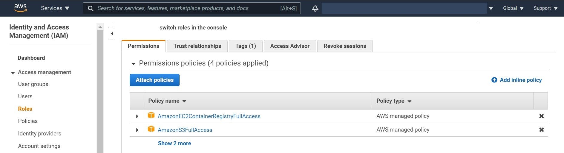
1. Permissions
To create and push the image to ECR, you need to give the required Permissions to the notebook instance. To do this, go to notebook instance configuration, and in the Permissions and encryption part, click on IAM role. After that, using the attach policy in the Permission tab, add SageMakerFullAccess and AmazonEC2ContainerRegistryFullAccess to the policies of this notebook.
2. Create ECR Repository
Now we can create the ECR repository to push our image to it using these bash scripts.
export REGION=eu-west-1
export IMAGE_NAME='your-desired-name'

aws ecr create-repository --repository-name $IMAGE_NAME --region $REGION
3. Building and Pushing Docker images to ECR
After creating the repository, we build the image according to our defined configuration in the Dockerfile and push it to the ECR repository:
export REGION=eu-west-1
export IMAGE_NAME='sktime-v4'
export ACCOUNT_ID=`aws sts get-caller-identity --query Account --output text`

docker build -t $IMAGE_NAME:estimator -f Dockerfile .

export IMAGE_ID=`docker images -q $IMAGE_NAME:estimator`

docker tag $IMAGE_ID $ACCOUNT_ID.dkr.ecr.$REGION.amazonaws.com/$IMAGE_NAME:estimator

aws ecr get-login-password --region $REGION | docker login --username AWS --password-stdin $ACCOUNT_ID.dkr.ecr.$REGION.amazonaws.com/$IMAGE_NAME:estimator

docker push $ACCOUNT_ID.dkr.ecr.$REGION.amazonaws.com/$IMAGE_NAME:estimator
Training the model
Here we copied a training script to our image that will be used in the training job. A sample training script is similar to script mode, but we don’t need to define the model_fn function here.
Initiating the training job
To start a training job, we need to define an Estimator object using our image. It’s similar to what we have done in script mode, except we need to pass our custom image URI to the Estimator object. This can be done with the following lines code:
import sagemaker
from sagemaker.estimator import Estimator

role = sagemaker.get_execution_role()

sk_training = Estimator(
             image_uri='your-image-address',
             role=role,
             instance_count=1,
             instance_type='ml.m5.large',
             output_path=output,
             hyperparameters={
                  'normalize': True,
                  'test-size': 0.1,
                  'random-state': 123})

sk_training .fit(inputs={'training':training})
Deploying the model
After the training job is finished, we can deploy our model to an inference instance so we’ll be able to send a request to it and get a real-time prediction. To do this, we use a simple Flask application that creates a REST API for our model to send predictions to the endpoint using a POST request. A sample serve script that can do this for us comprises of the following steps:
Loading the trained model
Defining a ping URL that SageMaker will use to make sure the inference instance is up and running
Defining an invocation URL that can get POST requests and use the trained model to return the prediction
Create the endpoint
The following code will deploy our trained model:
sk_predictor = sk_training .deploy(instance_type='ml.m5.large', initial_instance_count=1)

# set the predictor input/output configurations
sk_predictor.serializer = sagemaker.serializers.CSVSerializer()
sk_predictor.deserializer = sagemaker.deserializers.CSVDeserializer()
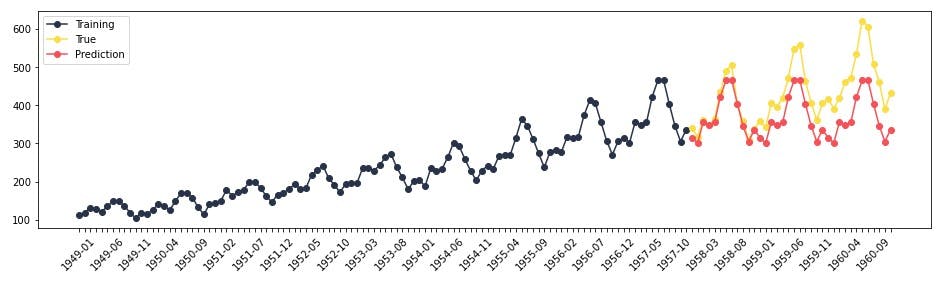
Now we can get some example predictions, and plot them:
import matplotlib.pyplot as plt
fig, ax = plt.subplots(figsize=(16, 4))

x = airline_dataset.iloc[:,0].values
y = airline_dataset.iloc[:,1].values
x_train = x[:-36]
x_test = x[-36:]
y_train = y[:-36]
y_test = y[-36:]
fh = np.arange(1, len(y_test) + 1)
y_pred = sk_predictor.predict(fh)
x_ticks = [x[i] if i%5 == 0 else '' for i in range(len(x))]

plt.plot(x_train, y_train, 'o-', c='#28334AFF', label='Training')
plt.plot(x_test, y_test, 'o-', c='#FBDE44FF', label='True')
plt.plot(x_test, y_pred, 'o-', c='#F65058FF', label='Prediction')

plt.xticks(x, x_ticks, rotation=45)
plt.legend()
plt.show()
Deleting the endpoint
After you are finished with the prediction, don’t forget to delete the inference instance. This can be done with the following code or manually through the AWS console (from SageMaker->Inference->Endpoints):
sk_predictor.delete_endpoint()
Conclusion
Here we described how to use the sktime package on Amazon SageMaker. We showed two approaches (script mode and docker mode) to train and deploy your sktime model. All of the codes and the notebooks from this blog post can be found in the DataChef GitHub repository.